SQL Server DO's and DON'Ts

 clipped from www.codeproject.com

SQL Server DO's and DON'Ts

So, you are now the leader of a SQL Server based project and this is your first one, perhaps migrating from Access. Or maybe you have performance problems with your SQL Server and don't know what to do next. Or maybe you simply want to know of some design guidelines for solutions using SQL Server and designing Database Access Layers (DAL): this article is for you.

Even if you are not using SQL Server, most of these design guidelines apply to other DBMS, too: Sybase is a very similar environment for the programmer, and Oracle designs may benefit from this too. I won't show here how to use specific T-SQL tricks, nor won't give you miracle solutions for your SQL Server problem. This is by no means a complete, closed issue. What I intend to do is give you some advices for a sound design, with lessons learned through the last years of my life, seeing the same design errors being done again and again.

DO know your tools.

Please, don't underestimate this tip. This is the best of all of those you'll see in this article. You'd be surprised of how many SQL Server programmers don't even know all T-SQL commands and all of those effective tools SQL Server has.

"What? I need to spend a month learning all those SQL commands I'll never use???" you might say. No, you don't need to. But spend a weekend at MSDN and browse through all T-SQL commands: the mission here is to learn a lot of what can and what can't be done. And, in the future, when designing a query, you'll remember "Hey, there's this command that does exactly what I need", and then you'll refer again to MSDN to see its exact syntax.

In this article I'll assume that you already know the T-SQL syntax or can find about it on MSDN.

DON'T use cursors

Let me say it again: DON'T use cursors. They should be your preferred way of killing the performance of an entire system. Most beginners use cursors and don't realize the performance hit they have. They use memory; they lock tables in weird ways, and they are slow. Worst of all, they defeat most of the performance optimization your DBA can do. Did you know that every FETCH being executed has about the same performance of executing a SELECT? This means that if your cursor has 10,000 records, it will execute about 10,000 SELECTs! If you can do this in a couple of SELECT, UPDATE or DELETE, it will be much faster.

Beginner SQL programmers find in cursors a comfortable and familiar way of coding. Well, unfortunately this lead to bad performance. The whole purpose of SQL is specifying what you want, not how it should be done.

I've once rewritten a cursor-based stored procedure and substituted some code for a pair of traditional SQL queries. The table had only 100,000 records and the stored procedure used to take 40 minutes to process. You should see the face of the poor programmer when the new stored procedure took 10 seconds to run!

Sometimes it's even faster to create a small application that gets all the data, proccess it and update the server. T-SQL was not done with loop performance in mind.

If you are reading this article, I need to mention: there is no good use for cursors; I have never seen cursors being well used, except for DBA work. And good DBAs, most of the time, know what they are doing. But, if you are reading this, you are not a DBA, right?

DO normalize your tables

There are two common excuses for not normalizing databases: performance and pure laziness. You'll pay for the second one sooner or later; and, about performance, don't optimize what's not slow. Often I see programmers de-normalizing databases because "this will be slow". And, more frequent than the inverse, the resulting design is slower. DBMSs were designed to be used with normalized databases, so design with normalization in mind.

DON'T SELECT *

This is hard to get used, I know. And I confess: often I use it; but try to specify only the columns you'll need. This will:

1. Reduce memory consumption and network bandwidth
2. Ease security design
3. Gives the query optimizer a chance to read all the needed columns from the indexes

DO know how your data will be/is being acessed

A robust index design is one of the good things you can do for your database. And doing this is almost an art form. Everytime you add an index to a table, things get faster on SELECT, but INSERT and DELETE will be much slower. There's a lot of work in building and mantaining indexes. If you add several indexes to a table to speed your SELECT, you'll soon notice locks being held for a long time while updating indexes. So, the question is: what is being done with this table? Reading or Updating data? This question is tricky, specially with the DELETE and UPDATE, because they often involve a SELECT for the WHERE part and after this they update the table.

DON'T create an index on the "Sex" column

This is useless. First, let's understand how indexes speed up table access. You can see indexes as a way of quickly partitioning a table based on a criteria. If you create an index with a column like "Sex", you'll have only two partitions: Male and Female. What optimization will you have on a table with 1,000,000 rows? Remember, mantaining an index is slow. Always design your indexes with the most sparse columns first and the least sparse columns last, e.g, Name + Province + Sex.

DO use transactions

Specially on long-running queries. This will save you when things get wrong. Working with data for some time you'll soon discover some unexpected situation which will make your stored procured crash.

DO beware of deadlocks

Always access your tables on the same order. When working with stored procedures and transactions, you may find this soon. If you lock the table A then table B, always lock them in this very same order in all stored procedures. If you, by accident, lock the table B and then table A in another procedure some day you'll have a deadlock. Deadlocks can be tricky to find if the lock sequence is not carefully designed.

DON'T open large recordsets

A common request on programming forums is: "How can I quickly fill this combo with 100,00 items?". Well, this is an error. You can't and you shouldn't. First, your user will hate browsing through 100,000 records to find the right one. A better UI is needed here, because you should ideally show no more that 100 or 200 records to your users.

DON'T use server side cursors

Unless you know what your are doing. Client side cursors often (not always) put less overhead on the network and on the server, and reduce locking time.

DO use parametrized queries

Sometimes I see in programming forums, questions like: "My queries are failing with some chars, e.g. quotes. How can I avoid it?". And a common answer is: "Replace it by double quotes". Wrong. This is only a workaround and will still fail with other chars, and will introduce serious security bugs. Besides this, it will trash the SQL Server caching system, which will cache several similar queries, instead of caching only one. Learn how to use parameterized queries (in ADO, through the use of the Command Object, or in ADO.NET the SqlCommand) and never have these problems again.

DO always test with large databases

It's a common pattern programmers developing with a small test database, and the end user using large databases. This is an error: disk is cheap, and performance problems will only be noticed when it's too late.

DON'T import bulk data with INSERT

Unless strictly necessary. Use DTS or the BCP utility and you'll have both a flexible and fast solution.

DO beware of timeouts

When querying a database, the default timeout is often low, like 15 seconds or 30 seconds. Remember that report queries may run longer than this, specially when your database grows.

DON'T ignore simultaneous editing

Sometimes two users will edit the same record at the same time. When writing, the last writer wins and some of the updates will be lost. It's easy to detect this situation: create a timestamp column and check it before you write. If possible, merge changes. If there is a conflict, prompt the user for some action.

DON'T do SELECT max(ID) from Master when inserting in a Detail table.

This is another common mistake, and will fail when two users are inserting data at the same time. Use one of SCOPE_IDENTITY, IDENT_CURRENT, and @@IDENTITY. Avoid @@IDENTITY if possible because it can introduce some nasty bugs with triggers.

DO Avoid NULLable columns

When possible. They consume an extra byte on each NULLable column in each row and have more overhead associated when querying data. The DAL will be harder to code, too, because everytime you access this column you'll need to check

I'm not saying that NULLs are the evil incarnation, like some people say. I believe they can have good uses and simplify coding when "missing data" is part of your business rules. But sometimes NULLable columns are used in situations like this:

CustomerName1
CustomerAddress1
CustomerEmail1
CustomerName2
CustomerAddress2
CustomerEmail3
CustomerName1
CustomerAddress2
CustomerEmail3

This is horrible. Please, don't do this, normalize your table. It will be more flexible and faster, and will reduce the NULLable columns.

DON'T use the TEXT datatype

Unless you are using it for really large data. The TEXT datatype is not flexible to query, is slow and wastes a lot of space if used incorrectly. Sometimes a VARCHAR will handle your data better.

DON'T use temporary tables

Unless strictly necessary. Often a subquery can substitute a temporary table. They induce overhead and will give you a big headache when programming under COM+ because it uses a database connection pool and temporary tables will last forever. In SQL Server 2000, there are alternatives like the TABLE data type which can provide in-memory solutions for small tables inside stored procedures too.

DO learn how to read a query execution plan

The SQL Server query analyzer is your friend, and you'll learn a lot of how it works and how the query and index design can affect performance through it.

DO use referential integrity

This can be a great time saver. Define all your keys, unique constraints and foreign keys. Every validation you create on the server will save you time in the future.

Conclusion

As I've said before, this is by no means a complete SQL Server performance and best practices guide. This would take a complete book to cover. But I really believe that this is a good start, and if you follow these practices, surely you will have much less trouble in the future.

Get Clipmarks - The easiest way to email text, images and videos you find on the web.

Calling a Web Service from an SQL Integration Services package

 clipped from www.codeproject.com

Calling a Web Service from an SQL Integration Services package

---

Introduction

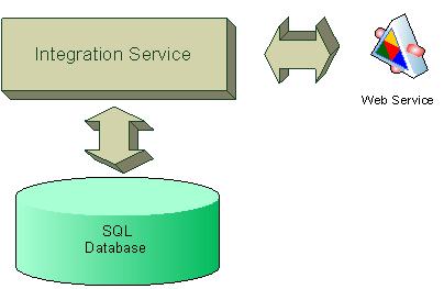
The SSIS framework provides the Web Service task which executes a Web service method. You can use the Web Service task for the following purposes:

• Writing to a variable the values that a Web service method returns.
• Writing to a file the values that a Web service method returns

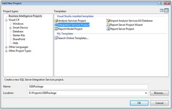
This article defines a step by step approach to use web service call in SQL integration services.

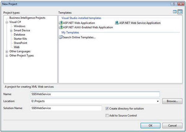
• Create a web service project

Figure 2 - Create Web Service

• Expose method call in the web service

    public class SSISService : System.Web.Services.WebService {         [WebMethod]         public string HelloMoon()         {             return "Hello Moon";         }         [WebMethod]         public int Multiply(int nParam1, int nParam2)         {             return nParam1 * nParam2;         } }

• Create SSIS package

Figure 3 - Create SSIS Package

• Add web service task

Figure 4 - SSIS Toolbox

Figure 5 - Web Service Task

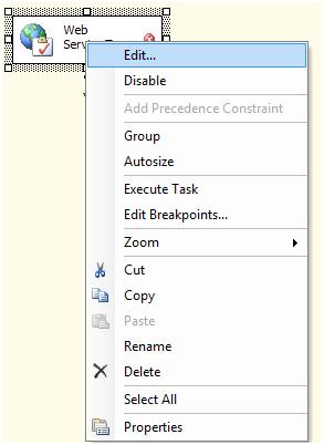
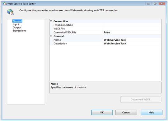
• Modify the web service task

Figure 6 - Edit Web Service Task

Figure 7 - Web Service Task Editor

• Define the HTTP Connection.

Figure 8 - HTTP Connection Manager Editor

• Define the WSDL File

Figure 9 - Web Service Task Edit (Definition of WSDL file)

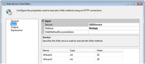
• Define the Web Service Task Inputs

Figure 10 - Web Service Task Editor (Definition of web service input properties

• Define the Web Service Output

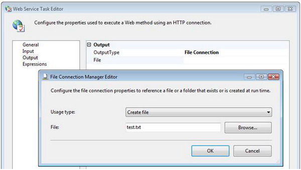
The output of the web service can be written to variables or output file. This sample outputs the results from the web service to a file system file that is defined using the File Connection Manager Editor (Figure 11)

Figure 11 - Web Service Task Editor (Definition of web service output properties)

Figure 12 - File Connection Manger

• Result

The following is the encoded output from the web service stored in the test.txt file.

<?xml version="1.0" encoding="utf-16"?>

<int>200</int>

References

[1] Web Service Task, SQL Server 2005 Books Online, http://msdn2.microsoft.com/en-us/library/ms140114.aspx

License

This article, along with any associated source code and files, is licensed under The Code Project Open License (CPOL)

Get Clipmarks - The easiest way to email text, images and videos you find on the web.

 clipped from www.sql-server-performance.com

Performance Tuning Tips for SQL Server BCP

By : Brad McGehee Jan 18, 2007

If you need to import or export very large quantities of data, it is often much faster to use bcp that it is to use DTS or SSIS. Of course, bcp lacks many features and options available for DTS and SSIS, and it a little more time-consuming to set up sometimes. But if you don't need to manipulate data, or if you deal with large amounts of data, or if you need a simple way to transfer data using a command line option, then you should investigate using bcp. [7.0, 2000, 2005] Updated 6-12-2006

*****

If appropriate, use the BCP native format instead of the character format to import and export data. It is much faster. Of course, this will limit you to BCP data between SQL Server databases with the same Character Sets and Dictionary Sort order. [6.5, 7.0, 2000, 2005] Updated 6-12-2006

*****

If appropriate, use the BCP fast mode to import data. The fast mode can save you substantial time for your data loads. Because there is no "fast mode" option to turn on, you must take all of the following steps to use the BCP fast mode:

·         The "select into/bulkcopy" database option must be set to "true".

·         The target table should not have any indexes.

·         The target table must not be published for replication.

·         Use the TABLOCK to lock the target table.

Get Clipmarks - The easiest way to email text, images and videos you find on the web.

SQL Server Query Optimization- Execution Plan

 clipped from www.sql-server-performance.com

SQL Server Query Execution Plan Analysis

By : Brad McGehee Apr 04, 2006

When it comes time to analyze the performance of a specific query, one of the best methods is to view the query execution plan. A query execution plan outlines how the SQL Server query optimizer actually ran (or will run) a specific query. This information if very valuable when it comes time to find out why a specific query is running slow.

There are several different ways to view a query's execution plan. They include:

• From within Query Analyzer is an option called "Show Execution Plan" (located on the Query drop-down menu). If you turn this option on, then whenever you run a query in Query Analyzer, you will get a query execution plan (in graphical format) displayed in a separate window.
• If you want to see an execution plan, but you don't want to run the query, you can choose the option "Display Estimated Execution Plan" (located on the Query drop-down menu). When you select this option, immediately an execution plan (in graphical format) will appear. The difference between these two (if any) is accountable to the fact that when a query is really run (not simulated, as in this option), current operations of the server are also considered. In most cases, plans created by either method will produce similar results.
• When you create a SQL Server Profiler trace, one of the events you can collect is called: MISC: Execution Plan. This information (in text form) shows the execution plan used by the query optimizer to execute the query.
• From within Query Analyzer, you can run the command SET SHOWPLAN_TEXT ON. Once you run this command, any query you execute in this Query Analyzer sessions will not be run, but a text-based version of the query plan will be displayed. If the query you are running uses temp tables, then you will have to run the command, SET STATISTICS PROFILE ON before running the query.

Of these options, I prefer using the "Show Execution Plan", which produces a graphical output and considers current server operations. [7.0, 2000] Updated 8-5-2005

*****

If you see any of the following in an execution plan, you should consider them warning signs and investigate them for potential performance problems. Each of them are less than ideal from a performance perspective.

• Index or table scans: May indicate a need for better or additional indexes.
• Bookmark Lookups: Consider changing the current clustered index, consider using a covering index, limit the number of columns in the SELECT statement.
• Filter: Remove any functions in the WHERE clause, don't include wiews in your Transact-SQL code, may need additional indexes.
• Sort: Does the data really need to be sorted? Can an index be used to avoid sorting? Can sorting be done at the client more efficiently?

It is not always possible to avoid these, but the more you can avoid them, the faster query performance will be. [7.0, 2000, 2005] Updated 8-5-2005

*****

If you have a stored procedure, or other batch Transact-SQL code that uses temp tables, you cannot use the "Display Estimated Execution Plan" option in the Query Analyzer or Management Studio to evaluate it. Instead, you must actually run the stored procedure or batch code. This is because when a query is run using the "Display Estimated Execution Plan" option, it is not really run, and temp tables are not created. Since they are not created, any references to them in the code will fail, which prevents an estimated execution plan from being created.

On the other hand, if you use a table variable instead of a temp table, you can use the "Display Estimated Execution Plan" option [7.0, 2000, 2005] Updated 8-5-2005

*****

If you have a very complex query you are analyzing in Query Analyzer or Management Studio as a graphical query execution plan, the resulting plan can be very difficult to view and analyze. You may find it easier to break down the query into its logical components, analyzing each component separately. [7.0, 2000, 2005] Updated 8-5-2005

*****

The results of a graphical query execution plan are not always easy to read and interpret. Keep the following in mind when viewing a graphical execution plan:

• In very complex query plans, the plan is divided into many parts, with each part listed one on top of the other on the screen. Each part represents a separate process or step that the query optimizer has to perform in order to get to the final results.
• Each of the execution plan steps is often broken down into smaller sub-steps. Unfortunately, they are displayed on the screen from right to left. This means you must scroll to the far right of the graphical query plan to see where each step starts.
• Each of the sub-steps and steps is connected by an arrow, showing the path (order) taken of the query when it was executed.
• Eventually, all of the parts come together at the top left side of the screen.
• If you move your cursor above any of the steps or sub-steps, a pop-up windows is displayed, providing more detailed information about this particular step or sub-step.
• If you move your cursor over any of the arrows connecting the steps and sub-steps, you see a pop-up window showing how many records are being moved from one step or sub-step to another step or sub-step.

Get Clipmarks - The easiest way to email text, images and videos you find on the web.

Cross Apply in SQL Server

Source Text at

A Visual Explanation of SQL Joins

I thought Ligaya Turmelle's post on SQL joins was a great primer for novice developers. Since SQL joins appear to be set-based, the use of Venn diagrams to explain them seems, at first blush, to be a natural fit. However, like the commenters
to her post, I found that the Venn diagrams didn't quite match the

SQL join syntax
reality in my testing.

I love the concept, though, so let's see if we can make it work. Assume we have the following two tables. Table A is on the left, and
Table B is on the right. We'll populate them with four records each.

id name       id  name
-- ----       --  ----
1  Pirate     1   Rutabaga
2  Monkey     2   Pirate

3  Ninja      3   Darth Vader
4  Spaghetti  4   Ninja

Let's join these tables by the name field in a few different ways and see if we can get a conceptual match to those nifty Venn diagrams.

SELECT * FROM TableA INNER JOIN TableB ON TableA.name = TableB.name id name id name -- ---- -- ---- 1 Pirate 2 Pirate 3 Ninja 4 Ninja Inner join produces only the set of records that match in both Table A and Table B.
SELECT * FROM TableA FULL OUTER JOIN TableB ON TableA.name = TableB.name id name id name -- ---- -- ---- 1 Pirate 2 Pirate 2 Monkey null null 3 Ninja 4 Ninja 4 Spaghetti null null null null 1 Rutabaga null null 3 Darth Vader Full outer join produces the set of all records in Table A and Table B, with matching records from both sides where available. If there is no match, the missing side will contain null.
SELECT * FROM TableA LEFT OUTER JOIN TableB ON TableA.name = TableB.name id name id name -- ---- -- ---- 1 Pirate 2 Pirate 2 Monkey null null 3 Ninja 4 Ninja 4 Spaghetti null null Left outer join produces a complete set of records from Table A, with the matching records (where available) in Table B. If there is no match, the right side will contain null.
SELECT * FROM TableA LEFT OUTER JOIN TableB ON TableA.name = TableB.name WHERE TableB.id IS null id name id name -- ---- -- ---- 2 Monkey null null 4 Spaghetti null null To produce the set of records only in Table A, but not in Table B, we perform the same left outer join, then exclude the records we don't want from the right side via a where clause.
SELECT * FROM TableA FULL OUTER JOIN TableB ON TableA.name = TableB.name WHERE TableA.id IS null OR TableB.id IS null id name id name -- ---- -- ---- 2 Monkey null null 4 Spaghetti null null null null 1 Rutabaga null null 3 Darth Vader To produce the set of records unique to Table A and Table B, we perform the same full outer join, then exclude the records we don't want from both sides via a where clause.

There's also a cartesian product or cross join, which as far as
I can tell, can't be expressed as a Venn diagram:

SELECT * FROM TableA
CROSS JOIN TableB

This joins "everything to everything", resulting in 4 x 4 = 16 rows, far more than we
had in the original sets. If you do the math, you can see why this is a very
dangerous join to run against large tables.

Database Snapshots and SSIS

clipped from blogs.conchango.com

Database Snapshots and SSIS

Did you think SQL Server 2005 database snapshots were really cool, but wondered how useful they were in practice? Building a Data Warehouse, here's an ideal use for them:

In my current project we're extracting data for the data warehouse from several SQL Server 2005 source system databases. Since we're extracting from multiple tables from each database, and since those tables continue to be populated during our extract, there is a definite risk that the extracted data is out of sync due to the extracts from different tables happens at slightly different times.

Database snapshots to the rescue

By first creating a snapshot of the source system database, and extracting from that static snapshot (instead of the original, changing database), these synchronization issues are avoided!

Even better, while the underlying database might be modified during the extract, the overhead for creating and using the snapshot is very small - it's proportional to the number of source system table pages changed during the extract.

Each source system database to be extracted has the following tasks configured:

1. The first Execute SQL Task creates the snapshot. Since no data is copied, this is a virtually instantaneous operation. At this stage the source system Connection Manager still points to the original database.

2. The first Script Task switches the database ConnectionString from the original database to the newly created snapshot database. This avoids having to create and keep a second connection manager in sync with the original database.

3. The Sequence Container contains all the Data Flow tasks etc. needed to move the source system data (now guaranteed to be static during the extract) into the data warehouse. NB: the following precedence constraints are "On Completion", so even if the extract fails, the snapshot will be deleted.

4. The second Script Task switches the ConnectionString back to the original database, i.e. almost same code as 2 above, but change "Source_System_Snapshot_Extract" into "Source_System", and vice versa.

5. The final Execute SQL Task simply drops the snapshot, again an instantaneous operation.

Wrapping up

One thing to watch out for is when additional database files are created, either manually by the DBA or automatically due to the source system having a maximum file size set. The snapshot creation command must specify ALL database files, so either update the snapshot command manually when this happens, or extend the Script Tasks to automatically figure out the number and filenames required.

In summary, database snapshots and SSIS have proved to be a very useful combination for extracting consistent data into the data warehouse.

Published 06 March 2006 18:45 by Kristian.Wedberg

Get Clipmarks - The easiest way to email text, images and videos you find on the web.

MDX at First Glance: Introduction to SQL Server MDX Essentials

www.databasejournal.com

MDX at First Glance: Introduction to SQL Server MDX Essentials

---

Unlock data warehouses with the analytical language of OLAP. Join Author Bill Pearson in the first of a new series of tutorials designed to get you up and running with the fundamentals of Multidimensional Expressions (MDX).

About the Series...

This is the first article of my new series, MDX Essentials. The primary focus of this series will be an introduction to the MDX language. The series is designed to provide hands-on application of the fundamentals of the Multidimensional Expressions (MDX) language, with each tutorial progressively adding features designed to meet specific real-world needs.

As we progress through the series, we will build upon previous lessons and the concepts we have introduced therein. However, one of my objectives is to make each lesson as "standalone" as possible, meaning that we should not encounter cases where we cannot complete a given lesson without components or objects that we have created in previous lessons. This should make it easier for "casual" visitors to join us with any lesson, and still successfully complete that session, given an existing understanding of concepts and principles that we have accumulated up to that point.

What We Will Need to Complete the Tutorials

To get the most out of the MDX Essentials series, we need to have installed at least the Analysis Services component of MSSQL Server 2000. While the full installation of SQL Server 2000 allows for virtually any exercise we might undertake, the majority of our sessions center on Analysis Services, the PivotTable Service, and their constituent parts. Installation of Analysis Services from the Standard Edition of MSSQL Server 2000 will be adequate for the vast majority of our activities.

For purposes of carrying out limited Microsoft Office -- related activities, Microsoft Excel 2000 and, to a lesser extent, Microsoft FrontPage 2000 will come in handy. We will also make use of the Microsoft OLAP Provider, included in a typical Excel 2000 installation, which consists of the data source driver and the client software needed to access cubes created by Microsoft SQL Server 2000 Analysis Services.

For purposes of the series, it is assumed that MSSQL Server 2000 and, specifically, the MSSQL Server 2000 Analysis Services components (I will often substitute the term "Analysis Services" going forward, to save time and space) are accessible to/installed on the PC, with the appropriate access rights to the sample cubes provided in a Typical installation of Analysis Services. It is also assumed that the computer(s) involved meet the system requirements, including hardware and operating systems, of the applications we have mentioned.

www.databasejournal.com

Introduction to MDX: The First Blush

This initial tutorial will introduce the MDX query in its simplest form. We'll take a look at some of the basic keywords, focusing only on simple queries, upon which we will build on in later lessons. Beginning in our first lesson, and throughout most of our series, we will discuss the element(s) of the language under consideration and then perform practice activities, with meaningful examples, to reinforce the concepts we have introduced. In this session, we will explore the rudiments of MDX queries within their simplest contexts (syntax) and introduce terms (semantics) that are applicable as they arise. This lesson will include:

• A brief introduction to MDX;
• A discussion of the basic keywords commonly used in MDX;
• A breakdown of a simple MDX query into its component parts;
• Brief comparisons and contrasts of MDX to SQL where useful;
• Other introductory items.

Let's begin by creating and executing a basic MDX query that will provide us a tangible starting point for discussing keywords and components.

Multidimensional Expressions (MDX) as a Language

MDX emerged circa 1998, when it first began to appear in commercial applications. MDX was created to query OLAP databases, and has become widely adopted within the realm of analytical applications. MDX forms the language component of OLE DB for OLAP, and was designed by Microsoft as a standard for issuing queries to, and exchanging data with, multidimensional data sources. The language is rapidly gaining the support of many OLAP providers, and this trend is expected to continue.

The focus of the MDX Essentials series will be MDX as implemented in MSSQL 2000 Analysis Services. MDX acts in two capacities within Analysis Services: as an expression language that is used to calculate values, and as a query language that is accessed and used by client applications to retrieve data. We will address aspects of both perspectives throughout the series.

The Basic MDX Query

Let's begin by creating a rudimentary query using the MDX Sample Application. The Sample Application is installed with Analysis Services and allows us to create an MDX statement, execute it, and see the results in a grid-like results pane. We'll start the application and proceed, taking the following steps:

1. Go to the Start button on the PC, and then navigate to Microsoft SQL Server -> Analysis Services, then to the MDX Sample Application.
2. We are initially greeted by the Connect dialog, shown in Illustration 1 below.

Illustration 1: The Connect Dialog for the MDX Sample Application (Enlarge)

The illustration above depicts the name of one of my servers, RAPHAEL, and properly indicates that we will be connecting via the MSOLAP provider (the default).

3. Click OK.

(We might also choose to cancel the dialog box and connect later by clicking Connect on the File menu.)

The MDX Sample Application window appears.

4. Clear the top area (the Query pane) of any remnants of queries that might appear.
5. Ensure that FoodMart 2000 is selected as the database name in the DB box of the toolbar.
6. Select the Warehouse cube in the Cube drop-down list box.

The MDX Sample Application window should resemble that shown below, complete with the information from the Warehouse cube displaying in the Metadata tree (in the left section of the Metadata pane between the Query pane at the top of the application window and the Results pane at the bottom.).

Illustration 2: The MDX Sample Application Window (Compressed)

We type our MDX statements into the Query pane, as we shall see. Above the Query pane are the menu bar and toolbar. The Metadata pane allows us to visually inspect structural information about the selected cube. Syntax examples on the right side of this middle pane assist us in the creation of our statements. The Results pane at the bottom of the application window presents the output of our MDX queries. We will discuss various attributes of the MDX Sample Application where they are relevant to the exercises we undertake, but it is highly useful to explore the Books Online for a wealth of detail about the application.

We will begin with an example: We are asked by an information consumer to provide the total sales and total cost amounts for the years 1997 and 1998 individually for all USA-based stores (including all products). We are asked, moreover, to provide the information in a two-dimensional grid, with the sales and cost amounts (called measures in our data warehouse) in the rows and the years (1997 and 1998) in the columns.

1. Type the following query into the Query pane:

   --MDX01-1:  Basic Query SELECT {[Time].[1997],[Time].[1998]}ON COLUMNS, {[Measures].[Warehouse Sales],[Measures].[Warehouse Cost]}  ON ROWS FROM Warehouse WHERE  ([Store].[All Stores].[USA]) 

The diagram below labels the various parts of the query:

Illustration 3: Labeled Parts of a Basic MDX Query

The following general discussion items apply to the syntax above, and to MDX queries in general:

• The top line of the query is a comment. We will discuss comments later in the series, but suffice it to say for now that the two dashes (--) represent one of three typical ways to place a comment in MDX syntax, so that it is ignored when the MDX is parsed.
  I introduce this at the present stage because I like to "label" queries in this way as I create them, so as to make them easy to identify for reuse or review. This is particularly handy when using the Sample Application, because the application displays the initial characters of the query in the dropdown selector (labeled "Query:") to the right of the database ("DB:") selector in the toolbar. Selection of a given query from a query file is easy, therefore, given the use of intuitive names/descriptions in the top line of the syntax.
  
  

• The cube that is targeted by the query (the query scope) appears in the FROM clause of the query. The FROM clause in MDX works much as it does in SQL (Structured Query Language), where it stipulates the tables used as sources for the query.
  


• The query syntax also uses other keywords that are common in SQL, such as SELECT and WHERE. Even though there are apparent similarities in the two languages, there are also significant differences. A prominent difference is that the output of an MDX query, which uses a cube as a data source, is another cube, whereas the output of an SQL query (which uses a columnar table as a source) is typically columnar.
  It is important to realize that MDX's cube output allows us to place any dimension from the source cube onto any axis of the query's result cube. Many axes can exist, and it is often better to think in terms of "axes" than in "dimensions" (as is quite common among both developers and information consumers) when designing an MDX query. This is for two main reasons: The "axes" concept allows for distinction between the source dimensions and the apparent result cube dimensions, which may be very different indeed. Another reason is that a given axis can contain a number of cube dimensions in combination. Axis references are therefore more precise, and less subject to misinterpretation.
  
  

• A query has one or more axes. The query above has two. (The first three axes that are found in MDX queries are known as rows, columns and pages.) We stipulate the axes above through our use of the "columns" and "rows" specifications. Keep in mind that columns always come before rows, and rows always precede pages, within the query.
  


• Curled brackets "{}" are used in MDX to represent a set of members of a dimension or group of dimensions. The query above has one dimension each on the two query axes. The dimensions that appear are the Measures and Time dimensions.
  


• We can display more than one dimension on a result axis. When we do this, an "intersection" occurs, in effect, and each cell appearing in the associated axis relates to the combination of a member from each of the indicated dimensions. When more than one dimension is mapped onto an axis, the axis is said to consist of "tuples," containing the members of each of the mapped dimensions.
  


• Dimensions that are not specified within the axes of a query will have members specified by default; we can also stipulate such members in the WHERE clause, as shown in our query above.
  

2. Click the Run Query button (the button sporting the green, arrowhead-shaped icon -- a tool tip will alight when the cursor is placed upon the button to positively identify it for us).

We see the results below, which appear as soon as Analysis Services fills the cells that it determines to be specified by the query.

Illustration 4: The Initial Query Results

2. Save the query by selecting File -> Save As and call the file MDX01-1, as shown in the illustration below.

Illustration 5: Saving the MDX Query via the Save As Dialog

Note: I typically prefer to save files to a context-oriented directory/folder (for example a folder I have created for a client for whom I am writing MDX queries as a part of an engagement, or for a presentation I am assembling). This is obviously a point of personal taste; the objective is simply to keep track of where the queries are, so that we can find them in time of need. Much rewriting and confusion between altered versions can be avoided by storing the queries in a logical system of some sort to keep organized. My favorite way to do this is to create a database within which to store the query strings, together with descriptions, author and keyword information, along with date time data, "version" information, and other specifics, if applicable.

Let's create another query to conclude this introductory session. This time, let's say that information consumers have asked for a comparison between the total US warehouse sales for the first and second quarters of 1997. We will again create a query against our Warehouse cube to generate this information.

1. Click the New Query button (depicted in the illustration below).

Illustration 6: The New Query Button

We might also have selected File -> New from the top menu.

2. Type the following query into the Query pane:

   --MDX01-2:  Basic Query 2  SELECT  {[Time].[1997].[Q1],[Time].[1997].[Q2]}ON COLUMNS,  {[Warehouse].[All Warehouses].[USA]}  ON ROWS  FROM Warehouse  WHERE  ([Measures].[Warehouse Sales]) 

Because we have specified the Warehouse Sales measure in the WHERE statement, we have made it the slicer dimension. The slicer shows that we have picked only the Warehouse Sales measure from the measures dimension. We will work with slicer dimensions, as well as with the other components of the simple queries we have examined in this lesson (and far more), as we progress through the MDX Essentials series.

3. Click Query on the top menu, then select Run, as shown below:

Illustration 7: Select Run from the Query Menu

Alternatively, F5 or the Run Query button might be selected for the same effect.

We see the results below, which appear as soon as Analysis Services fills the cells specified by the query.

Illustration 8: The Query Results

4. Save the query as MDX01-2.
5. Exit the Sample Application.

Our intent with the above examples is to begin our exploration of MDX and to provide a first exposure to simple query structure. We will cover the details of the syntax and its arrangement, and a host of other considerations, as we progress through the series.

clipped from www.databasejournal.com

Next in Our Series...

With this tutorial article, MDX at First Glance: Introduction to MDX Essentials, we began the new MDX Essentials Series. Our objective in this lesson was to introduce the MDX query in its simplest form. We took a look at some of the basic keywords, focusing only on simple queries, as a basis upon which to build in later lessons. In this lesson, we began a discussion of the elements of the MDX language that will carry forward as we progress through the series, and then performed practice activities, as we will do throughout the entire MDX Essentials series, to reinforce the concepts we introduce.

We explored the rudiments of MDX queries within their simplest contexts (syntax), and introduced several terms (semantics) that were applicable as they arose. We provided a brief introduction to MDX, and then discussed several basic keywords commonly used in MDX. We examined a breakdown of a simple MDX query into its component parts, comparing and contrasting MDX to SQL where useful. Finally, we discussed other relevant introductory keywords and components throughout the lesson as part of creating and executing basic MDX queries.

In our next lesson, Structure of the MDX Data Model, we will introduce the MDX data model, together with numerous of its components. These components will include cubes, dimensions, and several other terms we have already exposed. We will focus on the composition and use of tuples and sets in detail, and provide hands-on exposure to these building blocks. Rules of syntax will be emphasized, and will provide a basis for more complex query building later in the series. Finally, we will step through practice exercises to demonstrate tangible results to reinforce our discussions with examples.

See All Articles by Columnist William E. Pearson, III

Discuss this article in the MSSQL Server 2000 Analysis Services and MDX Topics Forum.

MDX Essentials Series

Article 1: MDX at First Glance: Introduction to MDX Essentials
Article 2: Structure of the MDX Data Model
Article 3: MDX Operators: The Basics
Article 4: MDX Members: Introducing Members and Member
Article 5: MDX Member Functions: The "Family" Functions
Article 6: MDX Member Functions: More "Family" Functions
Article 7: MDX Member Functions: The Cousin () Function
Article 8: MDX Member Functions: "Relative" Member Functions
Article 9: MDX Time Series Functions, Part I: PeriodsToDate() and Kindred Functions
Article 10: MDX Time Series Functions, Part II: The OpeningPeriod () and ClosingPeriod() Functions
Article 11: MDX Time Series Functions, Part III: The LastPeriods() and ParallelPeriod() Functions
Article 12: Basic Set Functions: The Order() Function
Article 13: Basic Set Functions: The Union() Function
Article 14: Basic Set Functions: The Intersect() Function
Article 15: Basic Set Functions: The EXCEPT() Function
Article 16: Basic Set Functions: The Filter() Function
Article 17: Basic Numeric Functions: The Count() Function
Article 18: Basic Set Functions: The CrossJoin() Function
Article 19: Basic Set Functions: Subset Functions: The Head() Function
Article 20: Basic Set Functions: Subset Functions: The Tail() Function
Article 21: Basic Set Functions: Subset Functions: The Subset() Function
Article 22: Basic Member Functions: The .Item() Function
Article 23: Numeric Functions: Introduction to the AVG() Function
Article 24: Basic Set Functions: The EXTRACT() Function
Article 25: Logical Functions: The IsEmpty() Function
Article 26: String / Numeric Functions: Introducing the IIF() Function
Article 27: String / Numeric Functions: More on the IIF() Function
Article 28: The CROSSJOIN() Function: Breaking Bottlenecks
Article 29: Set and String Functions: The GENERATE() Function
Article 30: Enhancing CROSSJOIN() with Calculated Members
Article 31: Basic Set Functions: The TopCount() Function, Part I
Article 32: Basic Set Functions: The TopCount() Function, Part II
Article 33: String / Numeric Functions: The CoalesceEmpty() Function
Article 34: String Functions: The .Name Function
Article 35: String Functions: The .UniqueName Function
Article 36: Drilling Through with MDX: The DRILLTHROUGH Statement
Article 37: Set Functions: The DRILLDOWNMEMBER() Function
Article 38: Set Functions: The DRILLDOWNMEMBERTOP() and DRILLDOWNMEMBERBOTTOM() Functions
Article 39: MDX Set Functions: The DRILLUPMEMBER() Function
Article 40: MDX Set Functions: DrillDownLevel()
Article 41: Set Functions: The DrillDownLevelTop() and DrillDownLevelBottom() Functions
Article 42: Set Functions: The DrillUpLevel() Function
Article 43: MDX Set Functions: The ToggleDrillState() Function
Article 44: MDX Set Functions: The Distinct() Function
Article 45: MDX Operators: The IS Operator
Article 46: Other MDX Entities: Perspectives
Article 47: MDX Numeric Functions: The .Ordinal Function
Article 48: MDX Operators: The IsLeaf() Operator: Conditional Logic within Calculations
Article 49: MDX Operators: The IsLeaf() Operator: Conditional Logic within Filter Expressions
Article 50: Logical Functions: IsSibling(): Conditional Logic within Calculations
Article 51: Logical Functions: IsSibling(): Conditional Logic within Filter Expressions
Article 52: Logical Functions: IsAncestor(): Conditional Logic within Calculations
Article 53: MDX Clauses and Keywords: Use HAVING to Filter an Axis
Article 54: Logical Functions: IsAncestor(): Conditional Logic within Filter Expressions
Article 55: Logical Functions: IsGeneration(): Conditional Logic within Calculations
Article 56: MDX Scripting Statements: Introducing the Simple CASE Statement
Article 57: Logical Functions: IsGeneration(): Conditional Logic within Filter Expressions
Article 58: String Functions: The .Properties Function
Article 59: String Functions: The .Properties Function, Part II
Article 60: MDX Essentials: Set Functions: The MeasureGroupMeasures() Function
Article 61: Set Functions: The .AllMembers Function
Article 62: MDX Numeric Functions: The Max() Function
Article 63: MDX Numeric Functions: The Min() Function
Article 64: Set Functions: The AddCalculatedMembers() Function
Article 65: Set Functions: The StripCalculatedMembers() Function
Article 66: Intrinsic Member Properties: The MEMBER_CAPTION Property
Article 67: Intrinsic Member Properties: The MEMBER_KEY Property
Article 68: Intrinsic Member Properties: The MEMBER_NAME Property
Article 69: Intrinsic Member Properties: The MEMBER_UNIQUE_NAME Property

Get Clipmarks - The easiest way to email text, images and videos you find on the web.